8  Chi-Square

Two primary uses: Tests of independence of observations Goodness of fit Confusion matrix/contingency table: Create a table of observed frequencies Calculate column and row totals Create expected frequencies1 Calculate ∆2 b/w observed & expected Sum squared differences/expected2 Compare observed χ² to critical3

https://www.statsdirect.com/help/chi_square_tests/22.htm

https://www.youtube.com/watch?v=mSNoAODXD5c https://rforhr.com/disparateimpact.html

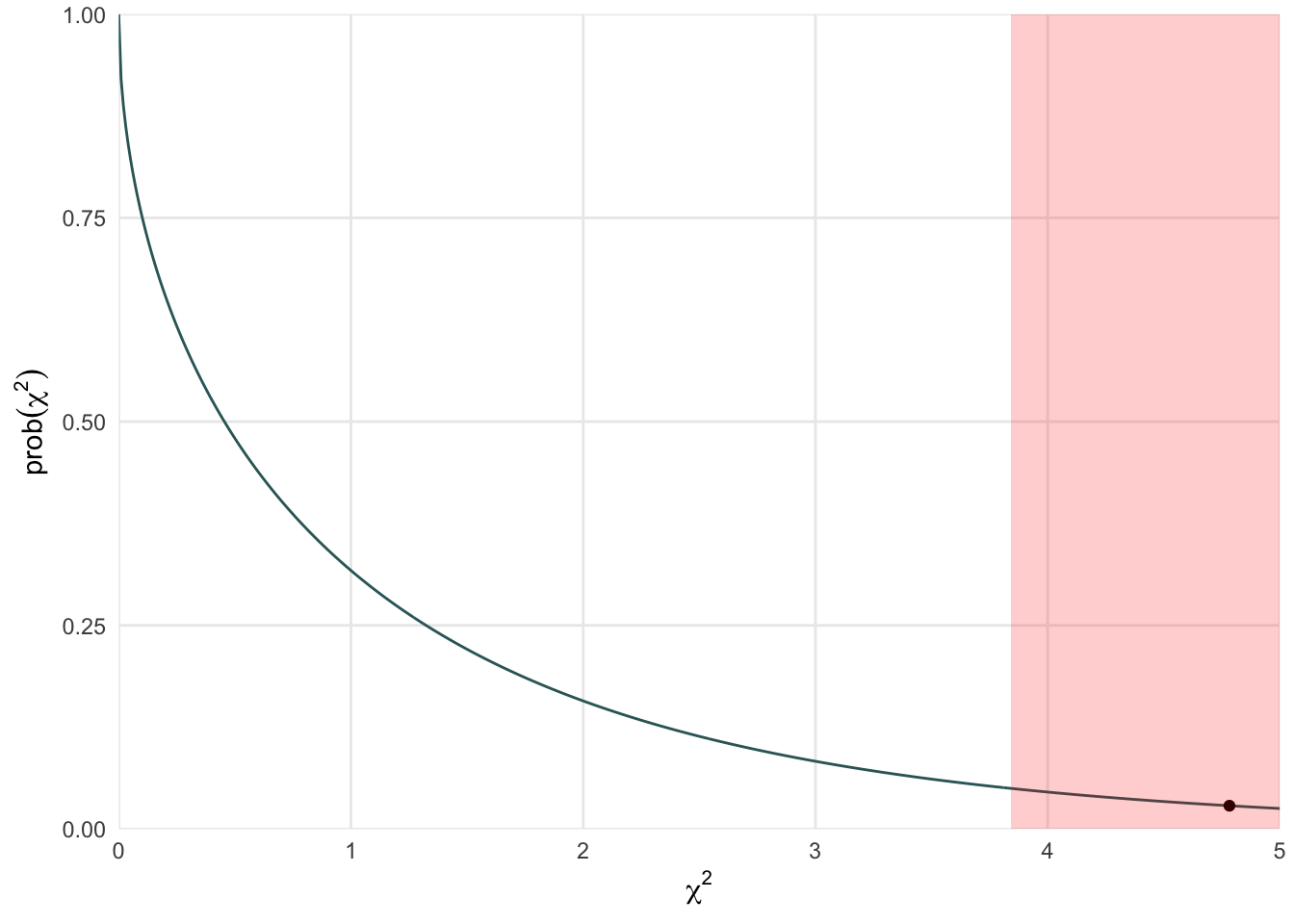
Expected is the (observed row sum * observed column sum)/grand total χ² formula = sum(Observed – Expected)^2/Expected) Can use observed matrix directing in R with {chisq.test(observed, correct=FALSE)} or calculate in Excel manually using {=CHISQ.DIST.RT(observed chi-square,1)} Males were not more likely than females to have passed the test, χ2(1) = 1.03, p = .31. Yates continuity correction accounts for the fact that 2x2 tables, as is the case here, tends to be upwardly biased, but it’s debatable if it needs to be applied. Fisher’s exact test is another test required when sample size is small (N < 30) but not often necessary as we typically work with larger sample sizes in IO. The critical value for a χ² with 1 degree of freedom is 3.84, so observed χ² values greater than this are statistically significant.

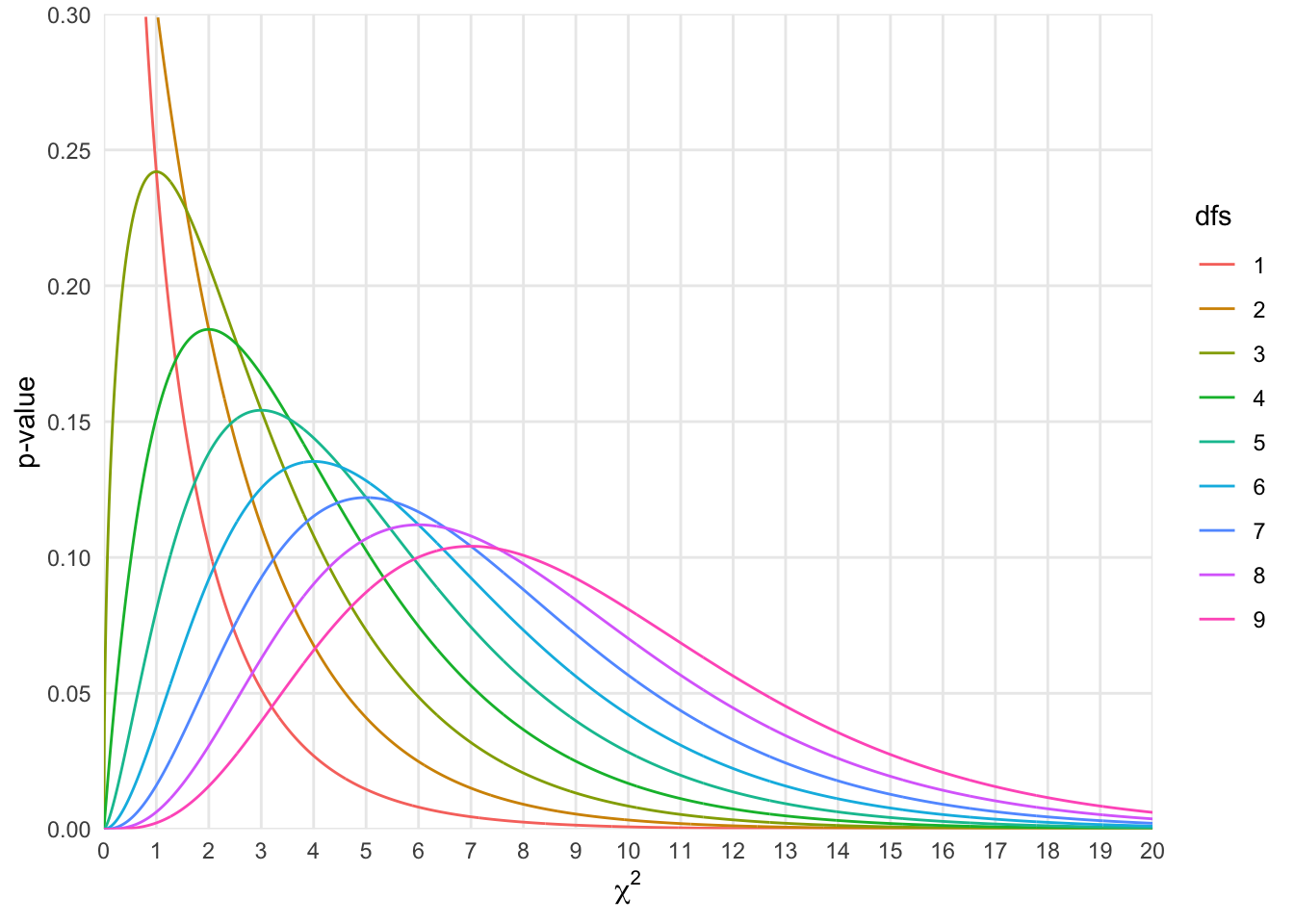
8.1 Chi-square (\(\chi^2\)) Distribution

Outliers: values outside the typical range of scores Skewness: measure of the asymmetry of a distribution Skewed distributions are common and violate statistical assumptions Lopsided distribution of values or scores influenced by outliers Negatively (left) skewed (e.g., job satisfaction ratings) Positively (right) skewed (e.g., income) Kurtosis: measures flatness/peakedness of the distribution

8.2 An Example

    Pearson's Chi-squared test

data:  observed
X-squared = 4.7826, df = 1, p-value = 0.02875

8.3 Calculating p-value

The p-value is calculated from the \(\chi^2\), where the values at 3.84 or greater are staistically significant. In this example, the obtained value is greater than the critical value.

8.4 Beyond the 2x2 Matrix

observed = matrix(data = c(58, 30, 50, 50, 24, 58), nrow = 2, ncol = 3, byrow = T)
observed

     [,1] [,2] [,3]
[1,]   58   30   50
[2,]   50   24   58

chisq.test(observed, correct=FALSE)

    Pearson's Chi-squared test

data:  observed
X-squared = 1.7194, df = 2, p-value = 0.4233

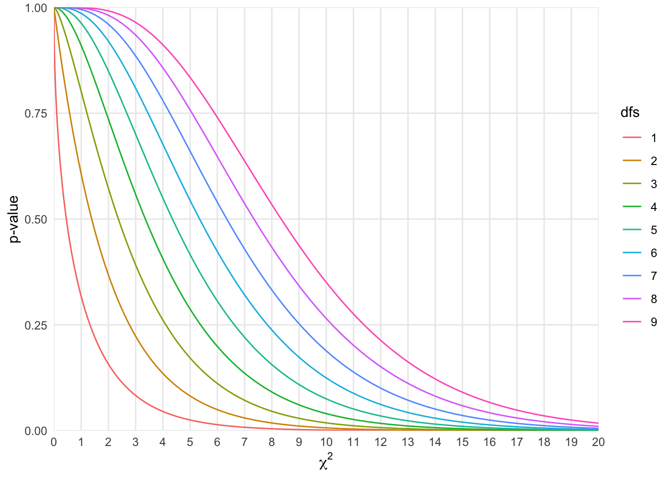
dfs <- 9
chi2 = seq(0,20,.01)
df_p <- matrix(ncol = dfs, nrow = length(chi2))

for(i in 1:dfs){
  df_p[,i] <- pchisq(chi2, df = i, lower.tail = F)
}

df_p <- data.frame(df_p)
colnames(df_p) <- 1:dfs
df <- cbind(chi2, df_p)
df <- gather(data = df, key = dfs, value = p, 2:10)

p <- ggplot(df, aes(x = chi2, y = p, color = dfs))
p <- p + geom_line()
p <- p + scale_x_continuous(name = expression(chi^2), expand = c(0,0), breaks = c(0:20))
p <- p + scale_y_continuous(name = "p-value", expand = c(0,0), limits = c(0,1), breaks = seq(0,1,.25))
p <- p + theme_minimal()
p <- p + theme(panel.grid.minor = element_blank()
)
p