12 Regression
12.1 Simple Linear Regression
Simple linear regression attempts to describe the relationship between one predictor and one criterion. There are five major #assumptions of a linear regression which required to be satisfied to ensure the results from the regression can be trusted in their interpretation and are not biased: 1. #linearity: this means the relationship between the predictor and the criterion is linear such that whenever the values on the predictor increase (decreases) the values in criterion always increase (decrease) at a consistent rate. This is contrasted from things like curvilinear or logistic relationships. 2. #autocorrelation: a lack of autocorrelation is assumed, meaning the residuals or prediction errors (the difference between the predicted value and actual value) are not related to one another. Auto correlation literally means data is correlated with itself. Autocorrelation may occur when repeated measures are used; for example, assume we asked job incumbents to take a test three times or in time series data. If people who score highly at time 1 are more likely to score highly on time 2 and then score higher on time 3. 3. #normality: multivariate normality means any random combination of predictors and criteria should be jointly, normally distributed. Multivariate normal looks like this . 4. #multicollinearity: a lack of multicollinearity is assumed as well, meaning predictors included in a multiple regression are not so correlated with each other as to be redundant. 5. #homoscedasticity: this assumption means the residuals are equal at every level of the independent variable.
12.1.1 Regression Elements
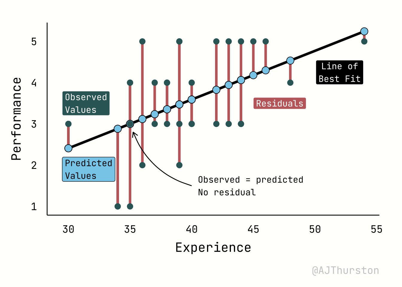
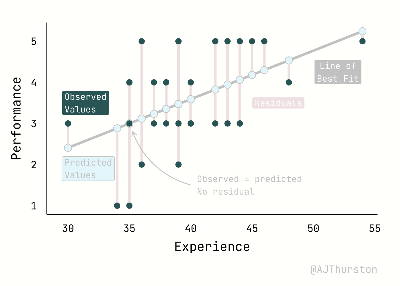
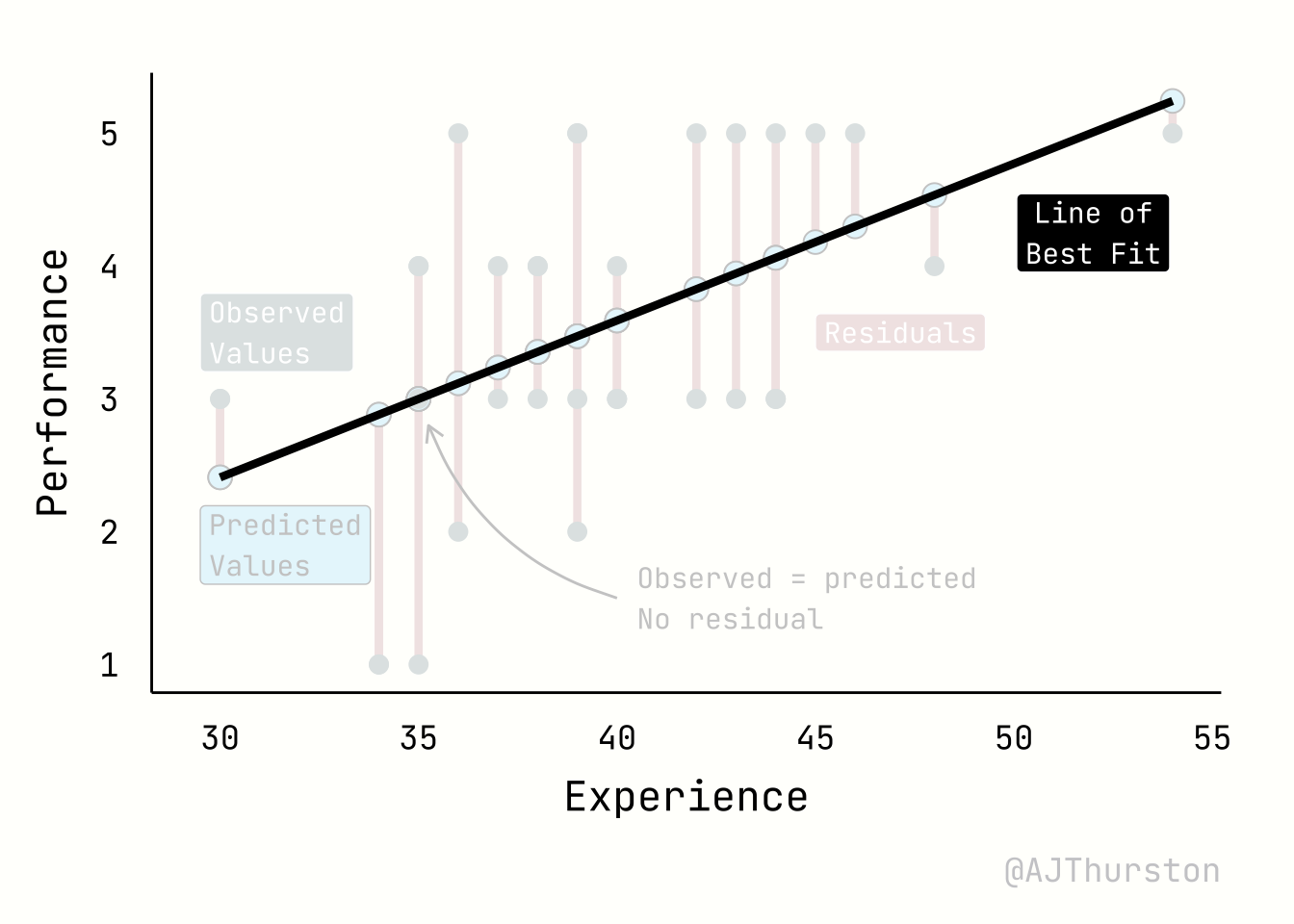
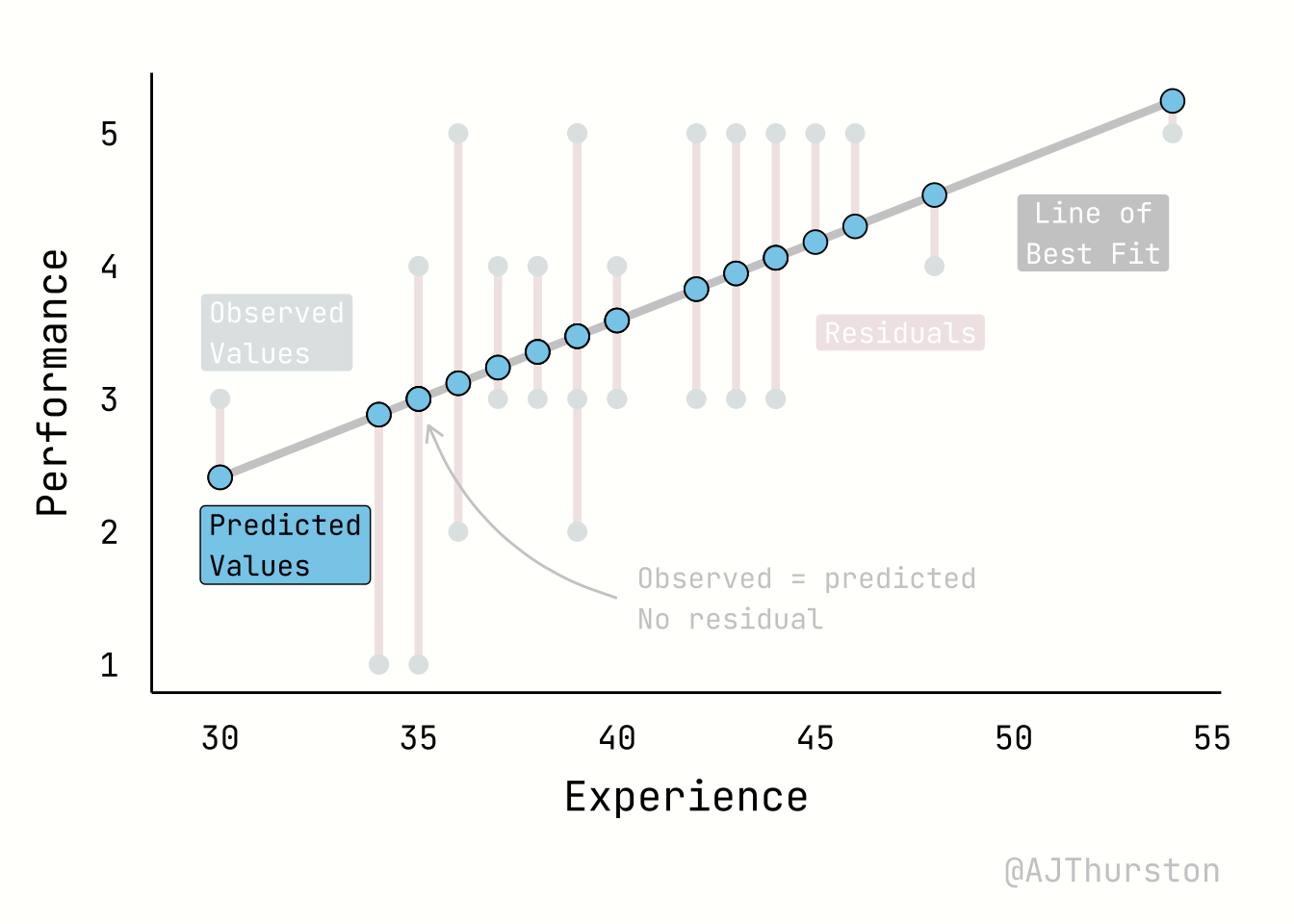
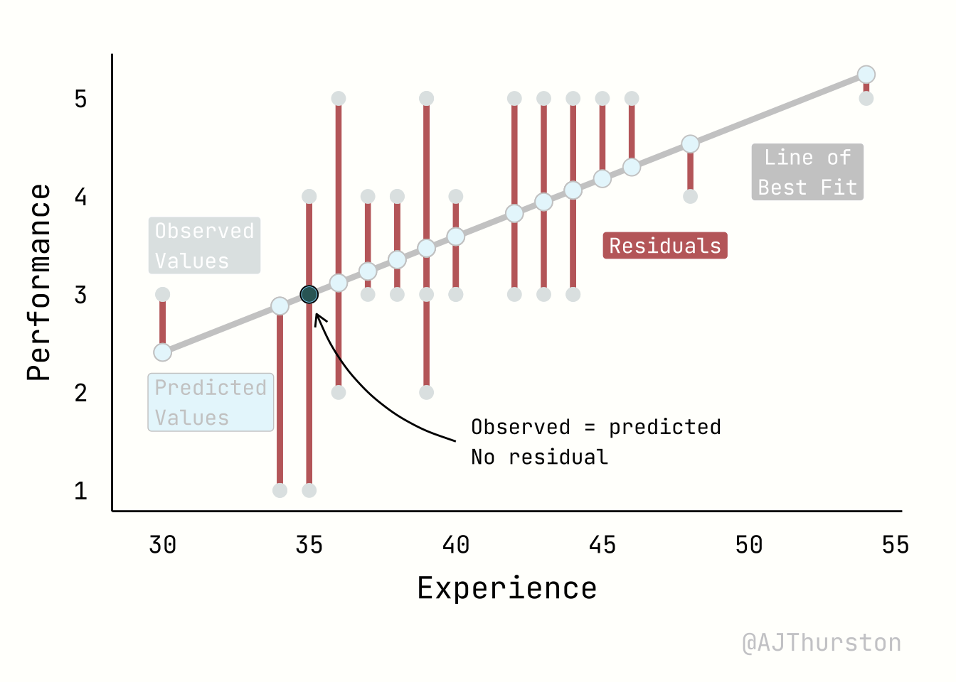
The regression plot below illustrates four core elements of a linear model: the regression line of best fit, the observed values, the predicted values, and residuals. The regression line represents the fitted relationship between experience and performance, estimated from the data by minimizing squared errors. The observed values are the actual data points, shown as individual markers scattered around the line. The predicted values are the locations on the line corresponding to each observed predictor value, reflecting the model’s best estimate of performance given experience. Residuals are the vertical distances between observed and predicted points, visualized here as line segments; they quantify the discrepancy between the model and reality, and together provide a visual measure of model fit.

12.2 Multiple Linear Regression (MLR)
Multiple linear regression is used when there are more than one predictor.
12.3 Regression diagnostics
- Variance Inflation Factor (VIF) and tolerance
- QQ (quantile quantile) plot
- Distance
- Fitted residuals
- Suppressor variables
12.4 Moderated Regression
- Need substantial power to detect moderator effects
- Often studies are underpowered to detect moderation (Aguinis et al., 2005)
- Should also be practically significant
12.4.1 Regions of Significance
- Pick a point analysis
- Johnson-Neyman technique (Johnson & Neyman, 1936; Bauer & Curran, 2005)
- Detailed expositions of the Johnson–Neyman technique are provided by Aiken and West (1991), Kerlinger and Pedhazur (1973), and Pothoff (1983).
Lin, H. (2020). Probing Two-way Moderation Effects: A Review of Software to Easily Plot Johnson-Neyman Figures. Structural Equation Modeling: A Multidisciplinary Journal, 27(3), 494–502. https://doi.org/10.1080/10705511.2020.1732826
Hayes, A. F., & Montoya, A. K. (2017). A Tutorial on Testing, Visualizing, and Probing an Interaction Involving a Multicategorical Variable in Linear Regression Analysis. Communication Methods and Measures, 11(1), 1–30. https://doi.org/10.1080/19312458.2016.1271116
Preacher, K. J., Curran, P. J., & Bauer, D. J. (2006). Computational Tools for Probing Interactions in Multiple Linear Regression, Multilevel Modeling, and Latent Curve Analysis. Journal of Educational and Behavioral Statistics, 31(4), 437–448. https://doi.org/10.3102/10769986031004437
https://www.ioatwork.com/test-bias-analysis-new-thoughts-on-an-old-method/
12.4.2 Simpsons Paradox
12.5 Generalized Linear Modeling (GLM)
Generalized linear regression attempts to describe relationships between variables when the relationship may or may not be linear. The GLM uses a more general form of the equation earlier, g(Y) = XB + e, where g() is the link function. The link function refers to the expected distribution of Y and maps a non-linear relationship to a linear one. By default the expected value of Y is the normal distribution as in simple linear regression, which is just a special case of the GLM.
There are many different linking functions:
Identity: This is the normal distribution used when the criterion is normally distributed.
Logit: This is used for binomial regression models, such as logistic regression. For instance, it could be used to predict whether an employee will leave or stay in the company (a binary criterion) based on their job satisfaction.
Log: This is used when modeling count data or rate data, often with a Poisson or negative binomial distribution. For example, it could be used to model the number of sales calls made by an employee in a day. There are other link functions within the GLM like the negative inverse for exponential distributions, the reciprocal, and the probit as the alternative to the logit which are not commonly used in I-O.
Logistic Regression
Polynomial Regression
Poisson Regression
On the other hand, the glm function fits models of a more general form, g(Y) = XB + e, where you need to specify both the function g() (known as the “link function”) and the distribution of the error term e. By default, glm uses the “identity function” for g(Y), which means g(Y) = Y, and it assumes a Normal distribution for the error term. In this default setting, glm essentially fits the same type of model as lm.
However, what makes glm “generalized” is its flexibility to handle models where the relationship between the predictors and the response is not strictly linear. This non-linearity is introduced through the chosen link function. Common examples of generalized linear models include Poisson regression and logistic regression. It’s worth noting that while “normal” regression is technically a type of generalized linear model, it’s often not referred to as such because it represents the primary and most common case upon which the general model framework is built.
12.6 Types of Regression
12.6.1 Simple Linear Regression
A simple linear #regression is the
12.6.2 Logistic Regression
- Predicted probabilites